
A search for the Standard Model Higgs boson via its decay to tau leptons and W bosons at the ATLAS detector

A search for the Standard Model Higgs boson via its decay to tau leptons and W bosons at the ATLAS detector
Understanding the origin or Electroweak symmetry breaking within the Standard Model was a key motivation for the construction of the Large Hadron Collider (LHC) experiment at CERN. This thesis presents a search for evidence of Higgs boson production in the 4.7 fb−1 of collision data recorded at a centre-of-mass energy of 7 TeV at the ATLAS detector during 2011.
This search is focused on signal events in which a Higgs boson is produced in the mass range 100 < mH < 180 GeV∕c2 and subsequently decays to a pair of W bosons or a pair of tau leptons to final states with one hadronically decaying tau lepton and one light lepton. After an event selection criteria has been applied, the number of events in this data sample is consistent with the total background estimate and an upper limit is placed on the SM Higgs boson production rate at 95% confidence level. In addition, the prospects for measuring the SM Higgs coupling strength to tau leptons with the associated Higgs production channels and the full LHC dataset are also presented.
Acknowledgements
Firstly I would like to thank my supervisors Sinead Farrington and Chris Hays for their support and seemingly in-exhaustible patience, particularly when I asked lots of silly questions. The past three years were made very pleasant by the past and present members of the Oxford ATLAS group for their help and useful suggestions; especially to James Ferrando and Hugo Beauchemin for sharing their expertise in the beginning and latterly to Elias Coniavitis for all of the invaluable conversations about the analyses we’ve worked on together.
I also owe a debt to the HSG4 group for their useful comments and suggestions, in particular to Sasha Prankho, Jed Biesiada, Elisabetta Pianori and Dimitris Varouchas.
To Alan Barr I also give credit, in particular for an insignificant conversation over lunch one day that quickly lead to a grant proposal and a successful outreach project for the Science and Technology Facilities Council with guidance from the ATLAS outreach group1 .
I’d also like to thank the other students of the Oxford ATLAS group2 , in particular Alex Pinder, Dan Short, Sam Whitehead, Caterina Doglioni, Phil Jones, Gemma Wooden, Aimee Larner and James Buchanan for all the laughter, and soothing words3 when things went wrong, particularly in the first year.
Contents
List of Figures
Chapter 1
Introduction
This thesis was submitted in the Spring of 2012, a few months before the observation of a new boson consistent with the decay of a Standard Model Higgs boson at mH = 125 GeV was jointly announced by the ATLAS and CMS collaborations.
The Large Hadron Collider (LHC) at the European Organization for Nuclear Research (known
as CERN) is the largest and highest energy particle collider in the world and has been regularly
colliding proton and lead-ion beams since November 2009. Collision events are recorded by the four
main LHC experiments: ALICE, ATLAS, CMS and LHCb. By the end of 2011, about
5 fb−1 of proton-proton collision data has been collected by both ATLAS and CMS at a
centre-of-mass energy  = 7 TeV, leading to the publication of many new search results
and measurements. The data collected to date represent a small fraction of the full
physics reach of the LHC which is expected to provide several hundred fb−1 of collision
data at
= 7 TeV, leading to the publication of many new search results
and measurements. The data collected to date represent a small fraction of the full
physics reach of the LHC which is expected to provide several hundred fb−1 of collision
data at  = 14 TeV. The analysis of these data is expected to expand the frontiers of
today’s knowledge of particle physics, which is condensed into the Standard Model
(SM).
= 14 TeV. The analysis of these data is expected to expand the frontiers of
today’s knowledge of particle physics, which is condensed into the Standard Model
(SM).
The SM of particle physics has been remarkably successful in explaining the results from decades of high energy physics experiments (including the LHC) in terms of elementary particles and their interactions. In spite of this, there are still as yet un-observed predictions of the SM: chief among them is the origin of particle masses. In the SM, particle masses arise through the so-called Higgs mechanism, evidence of which would be provided by the observation of the ‘Higgs boson’. The discovery of Higgs boson production in proton-proton collisions is one of the main goals of the LHC.
The results from previous direct searches, indirect SM measurements and theoretical arguments require the mass of the SM Higgs boson to be narrowly constrained where the LHC can observe it. However, to verify that an observed neutral resonance is indeed the result of Higgs boson production, its spin and coupling strengths to other SM particles must be measured and compared with the SM predictions.
The work in this thesis is dedicated to the analysis of data collected in 2010, 2011 and a feasibility study of measuring the Higgs boson coupling strength to tau leptons. Therefore, much work has been done to understand the tau identification algorithms used at ATLAS and in particular to measure the probability of mis-identifying a hadronic jet as a hadronically decaying tau lepton (the tau ‘fake rate’).
The outline of this thesis is the following: Chapter 2 gives an overview of the SM, the Higgs
mechanism and the physics of the Higgs boson at the LHC. A description of the LHC and the
ATLAS experiment is given in Chapter 3. In Chapter 4, a new application for visualising collision
events in ATLAS is described. A brief overview of tau lepton physics and an analysis measuring
the tau fake rate in ATLAS data collected in 2010 are described in Chapter 6. Chapter 7
documents two searches for a light SM Higgs boson using 2011 ATLAS data using final states with
a light charged lepton and a hadronically decaying tau lepton. In the absence of an observed
excess, an upper limit on the signal cross section is placed at a 95% confidence level for Higgs
boson masses in the range 100 < mH < 180 GeV∕c2. Finally, Chapter 5 presents the
prospects for measuring the Higgs boson coupling strength to tau leptons using events
in which the Higgs boson is produced in association with a weak gauge boson or a t
pair and subsequently decays to tau leptons, assuming 100 fb−1 of collision data at
 = 14 TeV.
Chapter 2
Theoretical overview 2.1 Introduction
This chapter gives a brief overview of the Standard Model, the Higgs mechanism and the phenomenology of Higgs boson production at a hadron collider.
The Standard Model (SM) [1, 2, 3] of particle physics is used to describe the fundamental, point-like constituents of matter and three of the four forces through which they interact: the electromagnetic (EM) and weak nuclear forces that can be unified into the electroweak (EW) force and the strong nuclear force which is described by the theory of quantum chromodynamics (QCD).
The SM is a relativistic quantum theory in which quantum fields are used to describe particles with spin 1/2 known as fermions, and integer spin particles known as bosons. The SM is a gauge theory based on the symmetry group SU(3)C ⊗ SU(2)L ⊗ U(1)Y in which interactions are introduced by requiring that the fermion fields remain invariant under a continuous group of local transformations. The dynamics of the fermion and boson fields are represented by a renormalisable Lagrangian
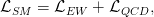 | (2.1) |
which is a function of these fields. This Lagrangian cannot be complete, however, since the QCD and electroweak interaction terms cannot account for the experimentally observed masses of the fundamental particles.
The Higgs mechanism extends the SM Lagrangian to include a scalar field and its interactions
 | (2.2) |
For a particular form of the scalar potential, this Lagrangian generates particle masses through the Higgs mechanism, also referred to as spontaneous symmetry breaking.
2.2.2 Particles of the Standard Model
Each particle field in the SM is defined by a unique set of quantum numbers. The twelve fermions, which are contained within three families of different flavour and increasing mass but otherwise identical quantum numbers, are shown in Table 2.2.2. For each fermion, there is a corresponding anti-particle with the same mass but opposite quantum numbers (such as the experimentally observed EM charge). Almost all visible matter in the universe is comprised of particles from Generation 1, since massive particles from higher generations are unstable. Fermions are further divided into leptons, which take part in electroweak interactions, and quarks that also participate in strong interactions due to their colour charge which can take three values: red, green and blue. Despite recent experimental results showing the neutrinos to have a tiny mass [4], in the SM they can be treated as massless. The boson particles that mediate the SM forces between the fermions are shown in Table 2.2.2.
| Fermions | Generations | Charge | Weak Isospin | Hypercharge | |||||||||||||||||
| 1 | 2 | 3 | Q[e] | T | T3 | Y | |||||||||||||||
| Leptons (L) |  |  |  |
|
|
|
|
||||||||||||||
| Leptons (R) | e | μ | τ | −1 | 0 | 0 | −2 | ||||||||||||||
| Quarks (L) |  |  |  |
|
|
|
|
||||||||||||||
| Quarks (R) |
|
|
|
|
|
|
|
||||||||||||||
| Bosons | Charge Q(e) | Mass (GeV) | Interactions |
| Photon: γ | < 5 × 10⁻³⁰ [6] | < 10−27 [6] | Electromagnetic: electrically charged particles. |
| Gluon: g | 0 | 0 | Strong: coloured particles (quarks and gluons) |
| W boson: W+,W− | ±1 | 80.385(15) [6] |
Electroweak:
fermions,
W,
Z,
γ
and
H. |
| Z boson: Z | 0 | 91.1876(21) [6] |
|
Electromagnetic and weak interactions are unified in the SM using the symmetry group SU(2)L ⊗ U(1)Y into electroweak interactions that distinguish between particles with left- and right-handed chirality. For a given generation, left-handed fermions manifest themselves as a doublet of leptons or quarks under actions of the SU(2)L group whose generator is the weak isospin operator, T. Weak Hypercharge, Y , is conserved quantity in electroweak interactions. The left- and right-handed fermions have different hypercharges under U(1)Y rotations. The non-zero masses of the W and Z bosons break the SU(2)L gauge symmetry, leaving a residual U(1)EM symmetry with electromagnetic charge Q, defined as
 | (2.3) |
.
The electroweak Lagrangian is given by
 | (2.4) |
where γμ are the Dirac matrices and L and R are the left- and right-handed projections of the fermion field. The four gauge fields, Wμi(i = 1, 2, 3) and B μ are related to the 3 + 1 degrees of freedom of the SU(2)L × U(1)Y group with the corresponding field strength tensors
 | (2.5) |
The covariant derivatives that preserve local gauge invariance are
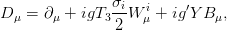 | (2.6) |
where σi(i = 1,.., 3) are the SU(2)L group generators (i.e. the Pauli Matrices) and g and g′ are coupling constants that determine the strength of the coupling to the SU(2)L and U(1)Y gauge fields, respectively. Since the Pauli matrices do not commute and the terms are non-Abelian, the Lagrangian contains self-interaction terms of the weak isospin gauge bosons.
The fields of the experimentally observable weak bosons Wμ±,Z μ and the photon Aμ are given by a linear combination of the electroweak gauge fields
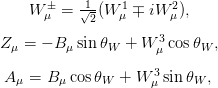 | (2.7) |
where θW is the weak mixing angle. The electric charge and electroweak couplings are also related by
 | (2.8) |
where the weak mixing angle has been measured experimentally using the Z pole observables; the Z-boson mass, mZ1 1and the Fermi constant which is derived from the muon lifetime formula. , to be sin 2θ W = 0.23146(12) [7] in the on-shell scheme and the strong coupling constant as measured at mZ, αs(mZ).
These transformed fields show that the charged W bosons couple to all left-handed fermions and right-handed anti-fermions with the same coupling strength. In the neutral-current interactions, the Z boson couples differently to each fermion depending on its charge and weak isospin.
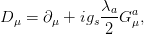
The strong nuclear interaction is based on the non-Abelian symmetry group SU(3)C and describes the interactions of particles that have colour charge, i.e. the quarks and gluons. Each quark forms a triplet in colour space that can have one of three colours with corresponding anti-colours for the anti-quarks (such that colour-anti-colour states are colour-neutral singlets). The group SU(3)C has eight generator matrices λa and hence there are eight different gluon gauge fields Gμa(a = 1,..., 8) where each is a unique colour-anti-colour superposition. The QCD Lagrangian is given by
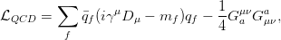 | (2.9) |
where qf and mf denote the quark fields and masses. In the QCD Lagrangian, the gluon fields enter via the field strength tensors
 | (2.10) |
where gs denotes the strong coupling constant and the structure constants fabc determine the commutators of the SU(3)C generators. The covariant derivatives that can be chosen to preserve local gauge invariance are given by
 | (2.11) |
and the local gauge invariance requires that the gluons are massless. The non-Abelian nature of this theory results in non-zero commutators of the generator matrices, resulting in cubic and quartic gluon self-coupling terms. These self-interactions also account for two phenomena of the quarks and gluons: the so-called ‘asymptotic freedom’ (that at very small length scales they can be regarded as free particles) and ‘confinement’ (observable particles are bound colour-singlets states and free quarks and gluons cannot be observed).
The EW and strong interactions of the SM so far require the particles to be entirely
massless2 2Even though mass terms are allowed for the fermion fields in  QCD, they are forbidden for the same fermion
fields in EW in order to conserve gauge invariance.
to ensure gauge invariance of the SM Lagrangian. This is completely at odds with a host of
experimental results in which the fermion and weak gauge bosons are shown to indeed have
mass.
QCD, they are forbidden for the same fermion
fields in EW in order to conserve gauge invariance.
to ensure gauge invariance of the SM Lagrangian. This is completely at odds with a host of
experimental results in which the fermion and weak gauge bosons are shown to indeed have
mass.
In the SM, particle masses can be introduced by a phenomenon known as the Higgs mechanism [8, 9, 10, 11] in which the mass terms are generated by spontaneously breaking the electroweak symmetry with a scalar field potential.
2.3.1 Spontaneous symmetry breaking
A complex, two-component scalar field,
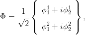 | (2.12) |
is introduced, chosen to be an isospin doublet of SU(2)L with weak hypercharge Y = 1. The self-dynamics of this new field are described by
 | (2.13) |
with the same covariant derivatives as for the EW Lagrangian shown in Equation 2.6. The scalar field potential is defined as
 | (2.14) |
If both λ > 0 and μ2 > 0 this potential takes the form shown in Figure 2.3.1 with a
continuous non-zero minimum at Φ†Φ = μ2∕2λ and a vacuum expectation value (VEV)
v =  .
.
The ground state of this field can be arbitrarily chosen along a ring of minimum potential, the act of which is known as spontaneous symmetry breaking. One choice is
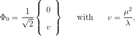 | (2.15) |
with an expansion around this ground state being described by
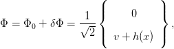 | (2.16) |
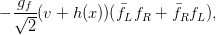
leading to a physical Higgs field h(x) (and three massless Goldstone bosons that are absorbed to give mass to the W± and Z gauge bosons). Substituting this into Equation 2.13 leads to terms where the Higgs field couples to the gauge fields WμiW iμ and B μBμ. A non-zero VEV produces mass terms for these gauge fields with eigenstates given by Equation 2.7 and eigenvalues given by
 | (2.17) |
The vacuum expectation value can also be calculated to be v = 246 GeV using the measured value of the Fermi constant [5].
To account for fermion masses, the Lagrangian is extended by the so-called ‘Yukawa’ terms
 | (2.18) |
Again substituting the expansion of the scalar field Φ around the chosen minimum leads to terms of the functional form
 | (2.19) |
in the Lagrangian from which the fermion masses can be read
 | (2.20) |
In the Lagrangian of Equation 2.13, one physical scalar field of the original four remains, the quantum of which is known as Higgs boson. As a consequence of this, if the Higgs mechanism describes the realisation of electroweak symmetry breaking in nature, there is a CP-even, electrically neutral particle that has coupling to all massive SM fermions and bosons that can be experimentally observed. However, the mass of the Higgs boson is not predicted in the Higgs mechanism and must be added by hand, i.e. it must be directly measured in an experiment.
2.4.1 Constraints on the Higgs mass
Terms in the electroweak Lagrangian (Equation 2.4) lead to vertices where the weak bosons self-interact. Since the probability for any processes cannot exceed one, a constraint on the s-wave scattering amplitude can be made such that as upper limit on the Higgs mass can be estimated: mH ≤ 850 GeV.
Another indirect constraint comes from the precision electroweak measurements observed at other experiments, with the Higgs boson mass left as a free parameter to be fitted. One example of this comes from the very well measured weak boson masses since the Higgs boson contributes to the W± vacuum polarisations through loop effects. Combining this with other electroweak measurements from LEP, SLC and the Tevatron leads to a fit value of mH = 87−26+35 GeV, or an upper limit of m H < 157 GeV at 95% confidence level [12].
The indirectly constrained range of Higgs masses is also consistent with the results from direct searches. If the global fit value takes into account the lower limit placed on the SM Higgs mass by the LEP experiments of mH > 114.4 GeV [12] then the indirect upper limit becomes mH < 186 GeV at 95% confidence level. The global minimum is shown in Figure 2.4.1.
Other direct searches conducted at the Tevatron analysing up to 10.0 fb−1 of p collision
data at a centre of mass energy  = 1.96 TeV exclude a 30 GeV wide mass region
around mH = 160 GeV in addition to the region already excluded by LEP, as shown in
Figure 2.4.1.
= 1.96 TeV exclude a 30 GeV wide mass region
around mH = 160 GeV in addition to the region already excluded by LEP, as shown in
Figure 2.4.1.
2.4.2 Production and decay at the LHC
At the LHC, there are several channels in which evidence of SM Higgs boson production can be sought. In particular, to identify any neutral resonance as a SM Higgs boson, its couplings to other SM particles and its spin must also be measured and compared with the SM predictions.
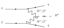
The mH dependence of the cross section for the dominant Higgs boson production processes is shown in Figure 2.5(a). The most abundant source is expected to be the gluon-gluon fusion process, the diagram of which is shown in Figure 2.4(a). It is the dominant production mode even though it is loop-induced because of the strong coupling of the Higgs boson to the (virtual) top quark, the relatively large αs for QCD processes and the huge flux of gluons at low Q2 for LHC collisions. Despite the lower cross section for vector boson fusion diagrams (see Figure 2.4(b)), it is expected that they provide a more sensitive search channel due to the lack of colour exchange between the out-going partons. Similarly, despite the lower cross section for the associated production diagrams shown in Figures 2.4(c) and 2.4(d), the additional final state particles from, for example, a leptonically decaying W boson, tend to completely change the background yield and composition.
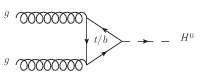
(a) Gluon-gluon fusion. |
(b) Weak boson fusion. |
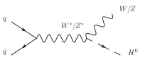
(c) Associated production with a weak boson. |
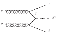
(d) Associated production with a t pair. |
In the SM, the coupling strength g of a Higgs to fermion anti-fermion (weak gauge-boson) pair vertex is directly proportional to the mass of the fermion (weak gauge-boson). The partial width of a Higgs to fermion anti-fermion (gauge-boson pair) decay Γf (ΓV ) is expressed
 | (2.21) |
The expected relative decay rate of a SM Higgs boson to a given pair of SM particles can be
expressed in terms of the branching ratio ( ). For a SM Higgs boson with a total decay
width Γtot and particular decay H → X with partial width ΓX the is defined to
be
). For a SM Higgs boson with a total decay
width Γtot and particular decay H → X with partial width ΓX the is defined to
be
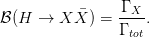 | (2.22) |
The total width increases rapidly as mH increases, with a jump of about three orders of
magnitude at the W+W− production threshold. For low masses preferred by fits to
electroweak data, Γtot << mH. The mass dependence of the of the Higgs boson is shown in
Figure 2.5(b).
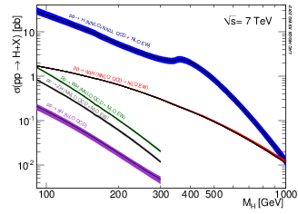
(a) SM Higgs boson production cross section at  = 7 TeV as a function of m
H. = 7 TeV as a function of m
H. |
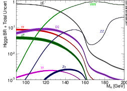
(b) Expected branching ratio of the SM Higgs boson to SM
particles as a function of the Higgs boson mass mH. |
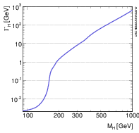
(c) SM Higgs boson total width as a function of mH. |
For a low-mass SM Higgs boson with 115 ≤ mH ≤ 135 GeV, the expected discovery modes are the subleading decays H → γγ, H → ZZ, and H → WW [15, 16, 17]. With more data, it is expected that the H → ττ and H → b [18, 19, 20, 21, 22] decays can be observed in various production processes, allowing a wide variety of Higgs boson cross section measurements. Specific SM Higgs boson coupling ratio measurements could then be made [23, 24] and compared with the SM prediction.
For masses favoured by global fits of electroweak data (mH < 135 GeV), the dominant decay mode is to b quarks, but due to the very high b jet production cross section at the LHC, this is experimentally very challenging. At these low masses, one of the most attractive decay modes to study becomes that to the heaviest leptons in the SM, tau leptons. At higher masses, another interesting decay mode with the same final state as a Higgs boson decaying to tau leptons is a Higgs boson decaying to a W+W− pair that subsequently decay leptonically with at least one W boson decaying to a tau lepton and a neutrino.
2.4.3 Measuring the SM Higgs boson coupling strength
With large LHC datasets (∫
 dt > 30 fb−1), it should be possible to measure the relative
coupling strength of Higgs to other SM particles by measuring the production cross section and
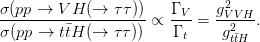
branching ratio of different Higgs production and decay processes. Cross section measurements are
proportional to the square of these couplings. For example,
dt > 30 fb−1), it should be possible to measure the relative
coupling strength of Higgs to other SM particles by measuring the production cross section and
branching ratio of different Higgs production and decay processes. Cross section measurements are
proportional to the square of these couplings. For example,
 | (2.23) |
where t is the top quark, V is a vector boson and ΓV and Γt are the partial widths of a Higgs to V or t decay.
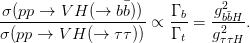
The ratio of two Higgs cross section measurements can be used as a direct probe of the ratio of the Higgs boson coupling strengths to such fields, for example
 | (2.24) |
or
 | (2.25) |
A ratio measurement has the advantage that some sources of systematic uncertainty common to both measurements will cancel when taken in ratio, for example the uncertainty on the integrated luminosity. Additionally, if both measurements have a common Higgs decay channel, systematic uncertainties on the measured Higgs decay products will also cancel.
Chapter 3
The ATLAS detector at the LHC 3.1 Introduction
In this chapter, a description of the LHC, the ATLAS1 1Formerly the experiment’s name was an acronym: A Toroidal LHC ApparatuS. detector and the event reconstruction algorithms used in the analyses presented in this thesis are given.
3.1.1 The Large Hadron Collider
The LHC [25] is a subterranean double-ring superconducting hadron collider, installed in
a circular tunnel of radius 4.25 km, located between 45 m and 180 m underground,
near Geneva, Switzerland. Eventually, proton-proton collisions are planned to have
 = 14 TeV and an instantaneous luminosity = 1034
cm−2s−1. The first successful
collisions occurred in Autumn 2009 at
= 14 TeV and an instantaneous luminosity = 1034
cm−2s−1. The first successful
collisions occurred in Autumn 2009 at  = 450 GeV. From March 2010 until the end of
2011, the first phase of the LHC physics research programme has been carried out with
collisions at
= 450 GeV. From March 2010 until the end of
2011, the first phase of the LHC physics research programme has been carried out with
collisions at  = 7 TeV, in which both the ATLAS and the Compact Muon Solenoid
(CMS) experiments have collected an integrated luminosity of about 5 fb−1. The lead ion
collisions are not discussed here, since they are not relevant for the analyses in this
thesis.
= 7 TeV, in which both the ATLAS and the Compact Muon Solenoid
(CMS) experiments have collected an integrated luminosity of about 5 fb−1. The lead ion
collisions are not discussed here, since they are not relevant for the analyses in this
thesis.
The LHC is designed to have up to 2808 circulating proton ‘bunches’, where each bunch has a diameter of about 7 μm and is made up of about 1011 protons. There is a spatial distance of about 7.5 cm between bunches or equivalently 25 ns between bunch crossings. Proton bunches are directed by 8.3 T magnetic fields generated locally by more than 1200 superconductive dipole magnets, each of which is about 15 m long. The beams are brought to collision at four points around the ring, where the four experiments ALICE, ATLAS, CMS and LHCb are situated in underground caverns, as shown in Figure 3.1.1.
On each side of the bunch crossing point, almost 400 quadrupole magnets 5-7 m long focus the proton bunches before collision. The LHC operates in ‘fills’ where protons are first accelerated from approximately at rest to 450 GeV, and then injected into the LHC. From there, it takes about 20 minutes for the beams to be accelerated to the target energy of the LHC in 2011: E = 3.5 TeV. Proton acceleration in the LHC occurs in eight superconducting radio frequency cavities around the ring, each with a field gradient of 5 MV∕m. After acceleration to 3.5 TeV, the beams are suitable for physics data for up to 10 hours, after which they are dumped onto an absorber and the next fill is prepared.
The coordinate system for events in the ATLAS detector is defined here and followed throughout the rest of this thesis. The counter-clockwise beam direction defines the positive z-axis while the x − y plane is transverse to the beam direction. The positive x-axis points towards the centre of the LHC ring and the positive y-axis points directly upwards. Switching to a cylindrical polar coordinate system, the polar angle θ and azimuthal angle ϕ are measured with respect to the z-axis and x-axis respectively. Since the polar angle θ is not invariant under a Lorentz boost, it is also useful to define the pseudo-rapidity of a particle with four-momentum (pX,pY ,pZ,E) as
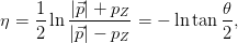 | (3.1) |
which is a measure of the ‘forwardness’ of a particle’s vector. A comparison of η and θ is shown in Figure 3.1.2.
The transverse momentum (pT) is defined to be the momentum in the plane transverse to the beam axis, i.e. the magnitude of the vector in the x − y plane. The angular separation of any two objects is also defined to be
 | (3.2) |
and is useful, for example, in removing overlapping reconstructed candidate objects or matching hits at the boundary between two sub-detectors.
3.1.3 Detector requirements and specifications
The ATLAS experiment [27, 28] is one of two general purpose experiments at the LHC and is designed in a layered configuration of nearly hermetic sub-detectors, as shown in Figure 3.1.3. ATLAS is intended to investigate a wide range of physical processes, some of which are shown in Figure 3.1.3.
ATLAS is therefore designed to handle more than 40 × 106 inelastic scattering interactions per
second, the vast majority of which are ‘minimum-bias’ events i.e. QCD interactions at
predominantly low momentum transfer. At = 1033 cm−2s−1 about 100 W and 10
Z gauge bosons are produced each second, with an expected Standard Model (SM)
Higgs boson production rate several orders of magnitude below this. The high rate for
weak boson production allows for an unprecedented increase in statistics from previous
experiments allowing precision measurement of quantities predicted in the SM. At the same
time, they also provide a significant source of background for SM Higgs searches. In
order to successfully perform measurements of high-rate processes in a high-luminosity
environment while also observing rare processes, the detector was designed with the following
requirements:
In order to make precise charge and transverse momentum measurements, there are two magnetic fields in ATLAS: a central solenoid (CS) and an air-core toroidal system.
The superconducting CS (shown in Figure 3.1.3) surrounds the inner detector and provides a 2 T magnetic field, causing the path of charged particles to follow a helix within its volume. From the curvature of this helix, precise charge and transverse momentum measurements can be made. A separate magnetic field of strength 0.5-1 T is created in the outermost region of the detector by three superconducting air toroids (again, shown in Figure 3.1.3). Like most of the sub-detectors, the air toroids are designed to cover the central (low |η|) area with a cylindrical ‘barrel’ module flanked at either end in the z-axis by two ‘endcap’ modules extending to higher |η|.
The inner detector (ID) consists of the tracking detectors surrounding the interaction point (IP) at the heart of ATLAS. The three sub-detectors that make up the ID: the pixel, semiconductor tracker (SCT) and transition radiation tracker (TRT) detectors are illustrated in Figure 3.3. As a charged particle propagates through these detector elements, space-point measurements are made while the path of the particle is bent by the CS magnetic field. From the curvature of the resulting helical path the particle describes, both the charge and the transverse momentum of the particle can be inferred.
To ensure good vertex reconstruction, the tracking detector closest to the IP requires the highest possible resolution to accurately extrapolate the reconstructed tracks back to the IP. In ATLAS, a silicon pixel detector based system is employed with three barrel layers arranged as concentric cylinders around the z-axis. In the higher |η| regions, two endcap modules consist of three disks placed perpendicular to the beam axis. The pixel detector provides an intrinsic position resolution of 10 μm in the R − ϕ plane and 115 μm in the z (R) plane in the barrel (endcap) region. In total, there are 1744 identical pixel elements with approximately 80.4 million readout channels.
In summary, a charged particle will produce up to three ‘hits’ in the pixel detector with very high spatial resolution that allow for primary and secondary vertex reconstruction, which can be used in b flavour jet and tau lepton tagging.
The ATLAS SCT barrel section comprises four cylindrical layers, each equipped with 8448 rectangular silicon-strip sensors. Both SCT endcap sections consist of nine disks such that any charged particle track with |η| < 2.5 will cross at least four of them (or the four barrel SCT layers). The silicon strips collect charge in a similar way to the pixel elements but with a coarser granularity, with an intrinsic resolution of 17 μm in the R − ϕ plane and 580 μm along the z (R) axis in the barrel (endcap) region. Each layer in the barrel and endcap is composed of two strip layers, crossed at a stereo angle of 40 mrad. The combination of measurements in the two strips provides a three dimensional position measurement of the traversed charged particle. In total there are about 6.4 million readout channels in the SCT.
3.3.3 Transition radiation tracker
The ATLAS TRT is the outermost radial ID sub-detector and performs measurements of tracks with |η|≤ 2 , providing a different approach to the silicon-based Pixel and SCT detectors.
The TRT is composed of 4 mm polyimide, straw drift tubes filled with a gas mixture of 3% O2, 27% CO2 and 70% Xe. These straws are situated parallel to the beam direction in the barrel region and radially in the endcap regions and hence only provide R − ϕ information, with an intrinsic resolution of 130 μm per straw. This lower resolution is mitigated by a large number of measurements per track, since each track will pass through ∼ 36 straws. In total, there are approximately 351,000 TRT readout channels.
Transition radiation is produced when a relativistic particle traverses an inhomogeneous medium such as the boundary between materials of different electrical properties. In the TRT, polypropylene fibres (foils) are situated between the barrel (endcap) straws to provide this boundary. The radiation produced ionises the gas mixture of the straw tubes. The resulting drift electron current is amplified by about a factor of 104 as it is drawn to a central gold plated tungsten wire running along the tube. The total drift time is approximately 40 ns.
The intensity of the radiation produced is proportional to the particle’s Lorentz factor γ = E∕m. Hence, due to the mass difference between electrons and charged hadrons, the magnitude of transition radiation can also be used to identify the track.
A more detailed view of the ATLAS calorimeters is shown in Figure 3.4. The main purpose of the calorimters is to determine the position and magnitude of energy deposited by particles. This is achieved using a highly granular liquid Argon (LAr) electromagnetic (EM) sampling calorimeter envelopes the solenoid with a central barrel section and two endcaps with coverage up to |η| < 3.2 and a hadronic calorimeter (HCAL) composed of different technologies for different regions of |η|, extending to a pseudo-rapidity of |η| = 4.9.
The energy resolution of the EM calorimeter is parametrised in terms of a so-called ‘sampling’
term2 2The sampling term has ∝ E1∕2 dependence due to the statistical nature of the energy deposition in the
calorimeters. and a
constant term3 3A constant term independent of E is also present due to non-uniformities in the detector calibration.
to be  =
=  ⊕ 0.0017 where ⊕ denotes addition in quadrature. The HCAL energy
resolution is parametrised to be
⊕ 0.0017 where ⊕ denotes addition in quadrature. The HCAL energy
resolution is parametrised to be  =
=  ⊕ 0.03.
The high granularity of the EM calorimeter is essential to the identification of electrons and photons. The coarser granularity of the HCAL is designed for jet reconstruction and measurements of an imbalance in the transverse momentum vector-sum of all energy deposits, the missing transverse momentum4 . The final function of the calorimeters is to contain the EM and hadronic shower shapes and hence limit any EM or hadronic particles from entering the muon detectors. This is accomplished with a minimum calorimeter depth of 22 interaction lengths (χ0) in the barrel region and 24 interaction lengths in the endcaps.
3.4.1 Electromagnetic calorimeters
The EM calorimeter consists of a central barrel section covering |η| < 1.475 with two endcap sections (1.375 < |η| < 3.2). The barrel is composed of two identical halves symmetric about z = 0, each made of 16 modules covering π∕8 of the ϕ plane. Each endcap has two coaxial wheels where the outer wheel makes precision measurements of particles with 1.375 < |η| < 2.5, and the inner wheel makes lower resolution measurements in the region 2.5 < |η| < 3.2. In the region designed to make precision measurements of photon and electron energy deposits, |η| < 2.5, the EM calorimeter is split longitudinally into three sections. The first is referred to as the ‘|η| strip layer’. The middle layer has a depth of 16 χ0, a coarser granularity than the |η| strip layer and is designed to contain the main energy deposit of an EM shower. The back layer is twice as coarse in granularity again and stops EM energy leaking into the hadronic calorimeter. To correct for energy losses in the dead material in front of the calorimeters, an additional thin liquid argon layer, the ‘presampler’ layer, sits in front of the η strip layer in the region |η| < 1.8. An illustration of the EM calorimeter is shown in Figure 3.4.1.
The EM calorimeter is a LAr sampling calorimeter with lead absorber plates that provide complete ϕ symmetry without any cracks in ϕ. The lead absorber plates also initiate electromagnetic showers of incident electrons and photons in which a cascade of EM particles is produced, starting from a single e+e− pair from a photon or a bremstrahlung photon ejected from an electron. Sandwiched between the lead absorber layers are LAr sampling layers in which the incident electrons ionise the Argon. The resulting charged current is collected by copper electrodes with a drift time of about 250 ns for a 2000 V potential.
The EM calorimeter energy resolution is parametrised after noise subtraction as:
 | (3.3) |
where a and b are constants describing the stochastic nature of the energy deposition and local non uniformities in the response, respectively. These constants have been measured as a function of |η| using electron test-beams with a known energy where a = 0.1 GeV1∕2 and b = 0.0017 for |η| = 0.69.
The hadronic calorimeter system measures the energy and direction of hadronic particles that survive the EM calorimeter. Hadronic calorimetry in the central region (|η| < 1.7) is provided by a plastic scintillator-tile sampling calorimeter (TileCal). In the TileCal, stacks of steel plates sandwiched with polystyrene scintillator tiles form the active material that initiate hadron showers. Each side of the scintillating tiles is read out by a photomultiplier tube.
At larger pseudo-rapidities up to |η| < 4.9, hadronic calorimetry is provided by the LAr Hadronic Endcap Calorimeter (HEC) and the Forward Calorimeter (FCal). The HEC is described above as the inner wheel of the EM endcap calorimeter. The FCal consists of three modules in each endcap. One is made of copper and is hence optimised for electromagnetic measurements whereas the other two are made of tungsten that is more suited to hadronic calorimetry. The total depth of the FCal is approximately ten interaction lengths.
The muon spectrometer forms the outermost layer of detectors around the IP, designed to measure the transverse momentum of charged particles with |η|≤ 2.7 that have passed through the calorimeters by measuring the curvature of their path as they pass though a non-uniform toroidal magnetic field. Due to the statistical nature of the energy deposition in the calorimeters there are rare so-called ‘punch through’ hadrons. These charged particles are almost always muons since they lose far less energy in the calorimeters.
The muon spectrometer is designed to provide a transverse momentum resolution of 10% for muon tracks with pT ≃ 1 TeV and make track pT measurements and identify the charge of tracks with pT ≤ 3 TeV. High pT leptons are a canonical event signature for many new physics models, including several Higgs boson analyses such as H → ττ → ℓνν τhν.
The layout of the muon spectrometer sub-detectors is shown in Figure 3.5. Precision track pT measurements are made by the monitored drift tube (MDT) chambers in the R − z plane with |η|≤ 2.7, the basic element of which is a pressurised drift tube with diameter 29.97 mm filled with an Ar∕CO2 gas mixture at 3 bar. An MDT chamber is composed of three to eight tubes with an average spatial resolution of 80 μm per tube. The innermost MDT barrel wheels are replaced by Cathode Strip Chambers (CSC) with a higher spatial resolution than the MDTs to better cope with the high particle fluxes at high |η|.
As charged particles traverse each tube the electrons produced from the gas ionisation are collected by a central tungsten wire held at a potential of 3080 V. The CSCs are multi-wire proportional chambers with radially aligned anode wires and perpendicular cathode strips that record hits by interpolating the charge from gas ionisation on adjacent cathode strips.
The muon spectrometer also has detectors with a lower pT resolution but with a much faster timing resolution of ≈ 4 ns used to make fast track pT measurements up to |η| < 2.4 in the muon trigger. Resistive Plate Chambers (RPCs) and Thin Gap Chambers (TGCs) are also present in the barrel and endcap regions, respectively.
The ATLAS detector is designed to record far fewer events for offline analysis than there are bunch crossings at even modest instantaneous luminosities. An event is categorised as interesting and hence worthy of recording offline by a three level system known as the ‘Trigger’. The Trigger is composed of a fast, online ‘level 1’ (L1) selection algorithm that passes event decisions to an offline ‘high level trigger’ (HLT) consisting of a ‘level 2’ (L2) and ‘Event Filter’ (EF) stage. When operating at the design luminosity of 1034 cm−2s−1, the event rate is expected to be approximately 1 GHz, of which about 200 Hz can be recorded offline. This requires the three stage trigger to reject approximately 5 × 10⁶ events per second. Since bunch crossings at the IP can occur every 25 ns, the system must make the decision quickly. A diagram of the ATLAS trigger and data flow model is shown in Figure 3.6.
For many analyses (including those described in this thesis), the hardware-based L1 trigger system is used to find high pT electrons, photons and muons. A reduced subset of the detectors including all the calorimeters and the muon RPCs and TPCs (but excluding the inner detector) is used to provide the L1 with this information with a lower resolution than is used in the offline selection. If a reconstructed object passing some pT threshold is found, this event is passed on to the HLT, otherwise it is discarded and no further attempt is made to record the event information.
After each bunch crossing, the detector information is time stamped and buffered into the pipeline memories located on the readout electronics (see Figure 3.6). The L1 trigger decision must reach the electronics within 2.5 μs of the bunch crossing. The detector electronics can handle a maximum event rate of 75 kHz.
Events selected by an L1 trigger are read out from the detector electronics into readout drivers (RODs) and then into readout buffers (ROBs) of which there are about 1700 in total. Intermediate buffers (‘derandomisers’ in Figure 3.6) are used to ensure the data can be read out of the pipeline memories with the available bandwidth of the RODs.
The HLT is entirely software based and processed on a dedicated farm of around 2000 computing elements using mostly commercially available hardware. Both the L2 and EF trigger algorithms use the full granularity of the calorimeter and muon sub-detectors combined with limited information from the inner detector.
All the detector data for a bunch crossing selected by the L1 trigger are held in the ROBs (see Figure 3.6) until they are either rejected by the L2 trigger or transferred to a storage area associated with the EF trigger. The L2 trigger receives so-called ‘Regions of Interest’ from the L1 algorithms that are geometric regions of the detector in which L1 physics objects have been identified. The L2 trigger runs more computationally intensive algorithms to further identify these objects with an average processing time of about 40 ms to reduce the event rate fed into the EF algorithms to about 3.5 kHz. The EF is a combination of offline algorithms that utilise the full detector information to decide which events are to be stored for further offline analysis at an expected rate of about 200 Hz5 , with an average processing time of about four seconds per event per computing node.
The ATLAS Data Acquisition System (DAQ) handles the intermediate buffering and data distribution. Events selected by EF trigger algorithms are written to a permanent storage site (Tier 0) located in the CERN computing centre. A second copy of every event selected by the EF algorithms is also stored at one of ten ATLAS Tier-1 sites, external to CERN to ensure data security. These data are later processed using higher level event reconstruction algorithms and stored in formats optimised for efficient user analysis and distributed via the ‘GRID’ using the file format of the ROOT analysis framework [31]. The GRID is a very large distributed network of computing and storage elements available to users for rapid data analysis through parallelisation of the analysis jobs.
Physics analyses of ATLAS data are based on the reconstruction of physics objects from detector information in the form of signals from the detector read-out electronics.
From the inner detector, hits recorded from the sub-detectors are reconstructed into helical tracks, the radius of which is determined by the particle’s pT and the magnitude of the magnetic field produced by the solenoid. These tracks are then extrapolated to the IP to reconstruct vertices, i.e. the common origin of two or more inner detector tracks. Electrons, photons, jets and hadronically decaying tau leptons are reconstructed using the tracks from the inner detector combined with energy measurements made in the calorimeters. Using the reconstructed vertex information, jets are further classified by a hypothesis of their origin from either a b or c hadron or a hadronic jet initiated by a light parton (u ,d , s quark or gluon).
To reconstruct muons, inner detector tracks are extrapolated to tracks reconstructed in the muon spectrometer. Since the incoming protons have no transverse momentum, the vector pT sum of all objects measured in the calorimeters and muon spectrometer is also used to measure the missing momentum or pmiss T vector. This is a measure of the negative vector pT sum of all particles produced in each collision that do not interact with any of the ATLAS sub-detectors, for example neutrinos produced in weak boson decay or uncharged particles from new physics models.
3.7.1 Inner detector track and vertex reconstruction
Inner detector tracks are reconstructed in an algorithm with three steps. First, hits in the silicon detectors and the TRT are used to build space-points. Second, the default tracking exploits the high granularity of the Pixel and SCT detectors to find tracks that can be extrapolated to the interaction region. In this step, track seeds are formed using space-points from the three pixel layers and the first SCT layer. These seed tracks are then extended to hits in the other SCT layers to form candidate tracks. Following this, each candidate is fitted to a hypothesis helix, outlier space-points are removed and any space-point-to-track ambiguities are resolved and fake tracks discarded by applying quality requirements. The surviving track candidates are then extended into the TRT and refitted using the full information of all three detectors.
Each reconstructed track can be parametrised by five quantities defined at the point at which the track is closest to the centre of the coordinate system. The quantities z0 and d0 denote the displacements between the centre of the detector and the point of closest approach along the beam axis and in the transverse plane, respectively. The angles ϕ and cot θ are the corresponding azimuthal angle and the cotangent of the polar angle. The other quantity is the ‘curvature’ of the helix, the inverse of the helix radius in the transverse plane, which is derived from the charge over the transverse momentum of the track, q∕pT. The measurement of these helix parameters is dependent on the number of multiple scattering interactions of the charged particle, and hence the amount of material traversed by the particle in the inner detector. The resolution of each parameter can be parametrised as a function of the track pT by
 | (3.4) |
where p′ is the pT at which the intrinsic and multiple scattering terms are equal for each parameter and σ(∞) is the resolution expected for a track of infinite momentum. Table 3.7.1 shows σ(∞) and p′ for each helix parameter in two regions of the detector in which different amounts of material have been traversed.
Helix parameter | 0.25 < |η| < 0.75 | 1.5 < |η| < 1.75
| ||
| σ(∞) | p′ (GeV) | σ(∞) | p′ (GeV) | |
| q∕pT | 0.34 TeV−1 | 44 | 0.41 TeV−1 | 80 |
| ϕ | 70 μrad | 39 | 92 μrad | 49 |
| cot θ | 0.7 × 10⁻³ | 5 | 1.2 × 10⁻³ | 10 |
| d0 | 10 μm | 14 | 12 μm | 20 |
| z0 × sin θ | 91 μm | 2.3 | 71 μm | 3.7 |
At the LHC, the nominal size of the bunches is σxy = 15 μm and σz = 5.6 cm, and so determining the coordinates of the primary interaction vertex (PV) along the z axis requires vertex reconstruction. In vertex reconstruction, reconstructed tracks are associated with a candidate vertex. In the vertex fitting step, the position of the PV is determined and parameters of the tracks of the associated tracks are recalculated, using constraints from the PV position. There are several vertex finding algorithms used in ATLAS but each is essentially finding the minimum of a χ2 function using the vertex position and the parameters of the tracks at a chosen vertex position.
3.7.2 Jet finding and heavy flavour tagging
To reconstruct the final state partons produced in each collision, jet finding algorithms are applied to the energy deposited in the calorimeters by the products of the parton hadronisation. In this thesis, every analysis uses an implementation of a sequential recombination algorithm, the anti-kt algorithm [32] that is both infrared and collinear safe, as shown in Figure 3.7.2.
The procedure for jet finding is:
![2 2 ΔR2ij 2 2 2
dij = min [(1∕pT)i,(1∕pT)j] × R2 with ΔR ij = Δ ϕij + Δ ηij](thesis71x.png) | (3.5) |
where R is a free parameter that determines the size of the jets, chosen in these analyses to be 0.4.
Clusters energies (and hence the final jet objects) are initially defined at the electromagnetic energy scale6 (EM scale)[33]. Corrections are made to account for the energy loss by particles traversing material in front of the calorimeter system and for deposits missed by the clustering algorithm.
In ATLAS, jet reconstruction is performed with a threshold of jet pT > 7 GeV. The free parameter R can be optimised for each analysis: small cone sizes acquire less contamination from objects close together in busy environments while larger cone sizes allow for a more precise energy resolution. Further quality criteria are required of the jet candidates in the H → ττ and H → WW∗ → ℓντν analyses (see Chapter 7).
Hadronic jets originating from b-quarks can be experimentally distinguished from jets originating from light partons. b-hadrons have a relatively long lifetime of τ ≈ 1.5 ps, so b-hadrons with high pT typically have a flight path in the transverse plane of several millimetres. The secondary vertex of the resulting jet can be identified by either reconstructing the decay vertex or combining the impact parameters of the charged hadron tracks into a discriminant [34].
In order to reconstruct electrons and photons, a ‘sliding window’ algorithm is used to look for EM calorimeter clusters produced by the electromagnetic particle showers. The algorithm is split into three steps: tower building, pre-clustering and cluster filling.
Initially, the calorimeter is segmented into a rectangular grid with Δη × Δϕ = 0.025 × 0.025 resolution. The window size of each reconstruction algorithm is shown in Table 3.7.4.
The energies deposited in every layer of a given geometrical unit of this grid are then summed to form an energy ‘tower’. For all towers with ET > 2 GeV, the electron reconstruction algorithm then attempts to match an inner detector track within a |Δη × Δϕ| window of 0.05 × 0.1. The ratio of tower energy to track momentum, E∕p, must be less than 10, and the tracks must not be consistent with γ → e+e− conversions. Energy corrections are made to account for energy loss due to bremsstrahlung in the inner detector. An electron candidate is created if an energy tower can be matched to a track, otherwise it is classified as a photon. In this way, approximately 93% of true, isolated electrons with pT > 20 GeV and |η| < 2.5 are reconstructed as electron candidates. Since on average an electron candidate will have shed 20% - 50% [27] of its energy (dependent on its |η|) after passing through the SCT due to bremsstrahlung and multiple scattering, energy calibrations are then applied to account for these additional particles which are collinear with the electron candidate.
Following this, the calibrated electron candidates are then subjected to dedicated identification algorithms to provide separation of true electron and photon candidates from hadronic backgrounds such as charged pions [35]. For electron candidates, three levels of quality, referred to as ‘loose’, ’medium’ and ‘tight’, correspond to decreasing levels of signal efficiency and simultaneously increasing levels of background rejection. The selection criteria for each level have been simultaneously optimised for up to seven η bins and up to six pT bins. The selection criteria for each are as follows:
Finally, a further cut is placed on the so called relative ‘isolation energy’ of the electron candidate which is defined as the energy sum of all additional EM calorimeter energy clusters within a cone of ΔR ≤ 0.2 of the candidate divided by the ET of the candidate, since hadronic backgrounds will usually be part of a wider hadronic jet. A similar cut is made relative to the candidate pT rather than an absolute cut on the isolation energy as it is more independent of the number of pileup interactions.
Two muon reconstruction and identification algorithms are used in ATLAS. So-called ‘standalone’ muon candidates are defined by a reconstructed track in the muon spectrometer with |η| < 2.7 extrapolated back to the beam line. ‘Combined’ muon candidates match reconstructed tracks in the muon spectrometer to reconstructed tracks in the inner detector and hence the pseudo-rapidity range is limited by the inner detector to |η| < 2.5. Despite the lower fiducial volume, the analyses described in Chapter 7 use combined muon candidates for the following reasons:
By using measurements from both detectors, the pT resolution is also improved. In the combined muon algorithm, a χ2 function is used to define how well a muon spectrometer track is matched to an inner detector track based on the outer and inner track segments or by partially refitting the helix parameters starting from the inner detector track and adding measurements from the muon spectrometer track, taking into account energy losses in material between the inner detector and muon spectrometer. Typically, the combined reconstruction algorithm will have a signal efficiency of about 94% for simulated single muons in a sample of the leptonic W boson decay and t production [27].
3.7.6 Hadronically decaying tau leptons
The first step in reconstructing hadronic tau decays (τh) is to ‘seed’ each reconstructed jet7 that has pT > 10 GeV and |η| < 2.5 as a candidate τh. Following this, the calorimeter clusters associated with the seed jet are refined and used to calculate kinematic quantities. Tracks reconstructed with the inner detector are associated with a τh candidate if they are reconstructed within a cone of radius ΔR = 0.2 from the seed jet axis and have:
where d0 and |z0 sin θ| are the track helix parameters described in Section 3.7.1. Tau candidates are then classified by the number of associated tracks, i.e. either single-prong or multi-prong for candidates with 1 or ≥ 1 track, respectively. A set of variables is then calculated from the tracking and calorimeter information. The variables are designed to provide good separation of hadronic tau decays from both hadronic jets produced in QCD interactions and electrons. The reconstructed variables are used to create a multivariate discriminant to reject backgrounds while accepting true τh.
A description of the τh identification algorithms and a data-driven analysis measuring the τh mis-identification rate at ATLAS are given in Chapter 6.
3.7.7 Missing transverse momentum
A large imbalance of transverse energy deposits in the calorimeters indicates the production of particles which have passed through the detectors without any interaction, such as neutrinos produced in the leptonic decay of a W boson. The missing transverse momentum is thus defined:
 | (3.6) |
In this definition, ∑
 T includes all energy deposits in the calorimeters and the
  T of reconstructed
combined muon candidates. Corrections are applied for energy clusters associated with identified
electrons, photons, muons, τh and jets [36]. Corrections are also made to account for gaps in
detector acceptance and additional detector material. Noisy electronics in the calorimeters are
also taken into account by only considering deposits above a cell’s noise threshold and
using clusters to which noise suppression cuts have also been applied, as described in
reference [27].
T of reconstructed
combined muon candidates. Corrections are applied for energy clusters associated with identified
electrons, photons, muons, τh and jets [36]. Corrections are also made to account for gaps in
detector acceptance and additional detector material. Noisy electronics in the calorimeters are
also taken into account by only considering deposits above a cell’s noise threshold and
using clusters to which noise suppression cuts have also been applied, as described in
reference [27].
In order for the Monte Carlo (MC) samples to provide an accurate description of what is observed in data, generated MC events must take into account the response of the detectors. The ATLAS detector simulation is performed with the GEANT4 [37] program using a detailed description of the material distributed in the ATLAS detector to simulate the full detector response, i.e. the signals provided by the detector electronics of the individual sub-detector modules. The particles produced in a MC event are propagated through the detectors and the simulation of the detector response is modelled using the GEANT4 program. The simulated detector signals are then passed through the full event reconstruction process, in the same way as is done for the real data taken from the experiment. Therefore, detailed studies of e.g. the electron and photon shower shapes and reconstruction efficiency are possible using simulated samples. However, it is often possible to calibrate such quantities in a data-driven way that is independent of MC, in case of any generator or simulation mis-modeling.
To study some systematic uncertainties, additional samples were created with deliberate detector misalignment introduced and slight distortions in the solenoid / toroidal magnetic fields to model the effect of a symmetry axis not coincident with the z-axis. Similarly, MC samples were simulated with additional non-active material in front of the calorimeters to better estimate the jet energy scale.
Chapter 4
Often in analysis, visual investigation presents a unique way in which to understand an aspect of detector performance or an event topology. With this in mind, a new tool that allows analysers to visualise ATLAS events on mobile platforms and devices has been developed.
4.2 Visualising ATLAS events on a mobile platform
LHSee [38] is an event display package developed to provide an interactive, visual investigation of both the ATLAS detector and the high-energy physics events it records. It is designed to be used on any mobile device using the Android operating system [39], including hand-held phones and tablet devices, with an intuitive and user-friendly interface to produce both 2-dimensional (2-D) projected visualisations and fully 3-dimensional (3-D) event displays which the average physicist or educator can easily interpret. LHSee implements several of the techniques first developed in the ATLAS event display programme ATLANTIS [40].
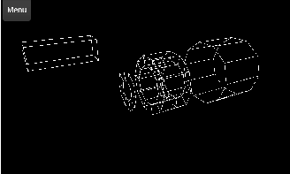
LHSee uses an implementation of the 3-D graphical application programming
interface OpenGLES [41] to render both the ATLAS detector and the event
information as a 3-D visualisation. The ATLAS detector can be visualised by first
defining a set of primitive geometrical shapes that can be thought of as embedded
graphs1 1A graph is composed of a set of vertices connected by a set of edges. For an embedded graph, each vertex also
has a position relative to the centre of the coordinate system. .
These graphs, shown in Figure 4.1, are then used with specific detector geometry information (first
implemented in ATLANTIS [40]) to build more complicated graphs that describe the various
ATLAS sub-detectors. In total,  (1000) vertices and edges are used to render the ATLAS detector
in each frame.
(1000) vertices and edges are used to render the ATLAS detector
in each frame.
 |
4.4 Visualising the detectors of the ATLAS experiment
The ATLAS detector and coordinate system are described in Chapter 3. LHSee can display projections of the various ATLAS sub-detectors that make up the inner detector in the plane parallel to the incoming protons (the z − y plane) and the plane perpendicular to the incoming protons (the x−y plane) as shown in Figure 4.2 and Figure 4.3, respectively. Alternatively, these detectors can also be visualised in 3-D, as shown in Figure 4.4, using the method described in Section 4.3.
The Electromagnetic and Hadronic calorimeters are represented as radial barrel components along the z-axis enclosing the inner detector, flanked on either side by endcap rings oriented perpendicular to the z-axis. This is shown in Figure 4.5, Figure 4.6 and Figure 4.7 with the Electromagnetic calorimeter in green, and the Hadronic calorimeter in red.
The sub-detector systems that make up the ATLAS Muon Spectrometer are collectively displayed in blue in both the 2-D projections and the 3-D visualisation, as shown in Figure 4.8 and Figure 4.9.
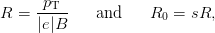
A charged particle passing through the inner detector travels along a curved path that can accurately be described by a helix, the radius of which is determined by the strength of the solenoidal magnetic field, the particle’s charge and its transverse momentum. To visualise charged particle tracks, points lying on each track helix are generated using a set of helix equations that can be parametrised for each track. The track helices are drawn from the closest point on the helix to the centre of the coordinate system to the point at which it leaves the inner detector fiducial region. Figure 4.3 and Figure 4.10 show the tracks from a simulated event in the projected plane transverse to the incoming protons and in 3-D in cyan and white, respectively.
Figure 4.11 shows the projection of a track helix in the x − y plane (i.e. a circle). The closest
point on this circle to the centre of the coordinate system, P0, is Pd with length D0 from P0. A
negatively charged particle travels along this circle in the anti-clockwise direction, initially in the
direction of ϕ0. The direction of the vertex as seen from the centre of the coordinate system P0 is
ϕ0 +  .
.
First, let us assume that the length of D0 = 0, and hence Pd = P0. The negatively charged particle will travel anti-clockwise along the circle with dα > 0 and dα increasing as it does so. This is defined as a positive turning circle with sign s = +1. A positively charged particle would have s = −1.
In a homogeneous solenoidal field, the radius of the circle, R, is inversely proportional to the strength of the magnetic field, B. According to the Lorentz force, R is given by
 | (4.1) |
where e is the charge of the particle. The centre of the circle Pc has coordinates (xc,yc) that are given by
 | (4.2) |
or
 | (4.3) |
If the circle does not pass through P0 and instead has a distance of closest approach D0 (see Figure 4.11), then these coordinates become
 | (4.4) |
as can be seen in Figure 4.11. The coordinates of the point of closest approach Pd are given by
 | (4.5) |
as shown in Figure 4.11. The coordinates of a point P on the circle at dα as seen from P are given by
 | (4.6) |
To turn this circle into a helix, a third coordinate is calculated in the z plane for every point on the circle, and is defined to be
 | (4.7) |
where z0 is the z coordinate of Pd and the tangent of the helix and the x − y plane is tan θ0 = pZ∕pT.
An embedded graph is created for each track using the five helix parameters (pT, e, cot θ0, ϕ0 and D0) in the following way:
This algorithm is used to define a graph for every reconstruced track in the event. Tracks with
pT greater than pT
Projections into the transverse plane of the energy deposited in the cells of the Electromagnetic
and Hadronic calorimeters with ET cell > 0.25 GeV are represented as histograms in the planes
transverse and parallel to the incoming proton beams. These histograms are superimposed directly
on top of the calorimeter visualisations, as shown in Figure 4.5 and Figure 4.6. The missing
transverse momentum vector,  T miss, is also represented in Figure 4.8 as a magenta arrow pointing
along the direction of the missing transverse momentum vector where the width of the arrow is
proportional to its magnitude.
T miss, is also represented in Figure 4.8 as a magenta arrow pointing
along the direction of the missing transverse momentum vector where the width of the arrow is
proportional to its magnitude.
A light-weight event display programme has been developed specifically to be used on mobile platforms that can be used to visually investigate the complex high-energy physics events that are recorded at the ATLAS detector at the LHC experiment and is freely available2 2https://market.android.com/details?id=com.lhsee . The intended primary use is as an educational tool and has been downloaded and installed by over 50,000 users worldwide.
Chapter 5
Expected Standard Model Higgs boson coupling measurements using the H →ττ channel 5.1 Introduction
At the LHC, the expected discovery modes for a light SM Higgs boson favoured by global fits of Electroweak data are the subleading decays H → γγ, H → ZZ, and H → WW [15, 16, 17]. However, to identify that a neutral resonance is consistent with a SM Higgs boson, its coupling strengths to other massive SM particles must be measured and compared with the SM predictions.
Extensive studies have been made of Higgs boson measurements at the LHC [42]. In this
chapter, a new study in presented of the sensitivity of 100 fb−1 of  = 14 TeV LHC data to the
associated Higgs boson production processes; WH, ZH, and tH, followed by H → ττ and at least
one W → lν or Z → ll decay. The production diagrams of these processes are shown in Figures
2.4.2(c) and 2.4.2(d).
= 14 TeV LHC data to the
associated Higgs boson production processes; WH, ZH, and tH, followed by H → ττ and at least
one W → lν or Z → ll decay. The production diagrams of these processes are shown in Figures
2.4.2(c) and 2.4.2(d).
Measurements in the associated production channels can be used to improve the LHC sensitivity to the coupling ratios gtH∕gZZH and gtH∕gWWH, the relevant ratio is
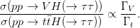 | (5.1) |
Furthermore, measurements in the H → ττ decay channels can be combined with the expected sensitivity of measurements of associated Higgs production cross section in the b decay channel [20, 21] to measure the Yukawa coupling ratio gHbb∕gHττ. This ratio is determined at leading order by the bottom-quark and tau-lepton masses and is sensitive to differences in the source of mass for quarks and leptons [43]. The relevant ratio measurements are
 | (5.2) |
This Chapter is structured as follows: Section 5.2 outlines the procedures for generating and simulating signal and background events; Section 5.3 describes the specific selection and expected signal and background yields for the WH, ZH, and tH processes; Section 5.4 details the cross section determination of each channel; Section 5.5 presents the expected coupling-ratio sensitivities and Section 5.6 summarises the conclusions.
5.2 Event generation and simulation
Monte Carlo samples of signal and background events are used to calculate event selection efficiencies and event yields. To account for detector acceptances and resolutions, a parameteric detector simulation is performed using Delphes.
Sherpa [44] is used to generate all signal and background MC samples used in Section 5.3 where possible, with parton distribution functions taken from CTEQ6L [45]. In these samples, tau leptons are decayed within Sherpa. In the tH analysis (Section 5.3.3), Alpgen [46] is used to generate the t + 2 jets and W + 6 jets background processes for the hard process and Pythia [47] is used for the hadronisation and showering due to the high multiplicity final states. For samples with jets in the final state, parton jets are included to leading order at the matrix-element level and additional jets modelled by parton showering within Sherpa and Pythia. The acceptances of Higgs-boson and diboson processes were cross-checked using the Herwig++ [48] event generator.
5.2.1 Parametric detector simulation
The Delphes simulation package [49] is used to model the detector geometric acceptance. Detector parameters are based on the ATLAS detector: the tracker is assumed to reconstruct all charged tracks with |η| < 2.5 with 100 % efficiency. Calorimeter towers cover the range |η| < 3.0 with electromagnetic and hadronic tower granularity of δη × δϕ ≃ 0.1 × 0.1, and cover the region |η| < 4.9 with coarser granularity. The energy of each stable particle is summed in the calorimeter tower through which it propagates. This energy, E, is then smeared according to Gaussian resolution functions assigned to the central, endcap and forward region electromagnetic calorimeters (EC) and hadronic calorimeters (HC) according to
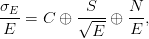 | (5.3) |
where E is expressed in units of GeV. The values used for the constant, C, sampling, S, and noise, N term of each sub-detector are chosen to match the expected performance of the ATLAS detector [33] and are shown in Table 5.1 along with the η region covered by each sub-detector.
| Detector | |η| | S (GeV )
) | N (GeV) | C |
|
EC | 0 − 1.7 | 0.101 | 0 | 0.0017 |
| 1.7 − 3.2 | 0.1 | 0 | 0.0017 | |
| 3.2 − 4.9 | 0.285 | 0 | 0.035 | |
|
HC | 0 − 1.7 | 0.5205 | 1.59 | 0.0302 |
| 1.7 − 3.2 | 0.70 | 0 | 0.05 | |
| 3.2 − 4.9 | 0.942 | 0 | 0.075 | |
The energy and pT of reconstructed electrons, muons, hadronically decaying τ leptons and jets are smeared according to Gaussian resolution functions matched to the performance of the ATLAS detector [33]. The acceptance criteria for these objects are summarised in Table 5.2.
In addition to the criteria listed in Table 5.2, a jet is only tagged as a hadronically decaying τ lepton if more than 90% of its energy falls within a cone of radius δR < 0.15, with one or three charged particle track(s) with pT > 2 GeV within a cone of radius δR < 0.4 from the jet axis.
The reconstruction of jets is performed using information from the calorimeter towers, with the anti-kt algorithm [32]. This algorithm is applied using the FastJet package [50], as implemented in Delphes. The b-tagging efficiency is assumed to be 60% for all jets with an associated generator level b-quark, with a b-tagging fake-rate of 10% for c-jets and 1% for light-quark or gluon jets. The jet acceptance is chosen to be conservative under high instantaneous luminosity conditions.
The dominant background to several signal channels consists of events where a light jet has been mis-identified as an e, μ or τh. In accordance with the description of the ATLAS detector given in [33], a separate identification efficiency and jet mis-identification rate is applied for each object. These values are summarised in Table 5.3.
To account for the effect of triggering, approximate trigger efficiencies given in [33] are applied for a single light lepton trigger to each analysis channel. The trigger efficiency for each, along with the minimum pT assumed for the trigger are listed in Table 5.4.
At high luminosity, the presence of pile-up events is expected to affect the detector response. At
an instantaneous luminosity of = 1034 cm−2s−1, one can expect ≃ 25 additional interactions
with ∑
ET = 30 GeV per interaction [30], where ∑
ET is the total ET measured in the
calorimeters. Since the pmiss
T resolution of ATLAS is predicted to be ∼ 0.5 [33], we smear
the projections pxmiss and p
ymiss with a Gaussian term, with a width of 10 GeV or 15 GeV. The
two choices correspond to an optimistic and nominal expectation of the pmiss
T resolution,
respectively.
[33], we smear
the projections pxmiss and p
ymiss with a Gaussian term, with a width of 10 GeV or 15 GeV. The
two choices correspond to an optimistic and nominal expectation of the pmiss
T resolution,
respectively.
It is also expected that at this high instantaneous luminosity the tau-ID efficiency will be significantly degraded. We therefore also use two scenarios of tau-ID performance: 40% efficient and 28% efficient, with a corresponding tau fake-rate of 1% [51].
5.3 Event selection and sensitivity
Subdividing the three production channels WH, ZH and tH by the decay of the tau leptons originating from the Higgs boson (i.e. hadronic or leptonic tau decay) leads to nine signal channels. For each decay channel, an event selection is applied to suppress the background in that channel. A one-dimensional binned-likelihood fit is then performed with a mass-based distribution of the surviving events to evaluate the channels’ sensitivity. By using a binned-likelihood fit, normalisation uncertainties on the background are constrained.
In the following sections, all reconstructed objects are required to pass the acceptance criteria listed in Table 5.2 and are assumed to be reconstructed and identified with the efficiencies listed in Table 5.3. Events are also required to have one lepton passing the single lepton trigger selection criteria described in Section 5.2.1. Tables and figures of expected signal and background contributions assume the ‘nominal’ conditions, in which the tau identification efficiency is expected to be 40% and the effect of pile-up on the pmiss T resolution is estimated by smearing the reconstructed px,ymiss with an additional Gaussian term of width 15 GeV.
In the WH channels, only events in which the W boson decays leptonically are considered. This leads to final states containing one lepton, pmiss T from the neutrino and two tau leptons from the Higgs boson decay. Events in which both tau leptons decay hadronically (H → ττ → τhτhνν) are not considered due to an overwhelming background contribution from W(→ ℓν) +jets production in which two jets have been mis-identified as hadronic tau decays (using a ≃ 1% tau fake-rate). Events in which both tau leptons decay leptonically are also not included since the branching ratio for ττ → ℓ+ℓ− 4ν is much lower than that of ττ → ℓτ h 3ν and the leptons from tau decay are less likely to pass the acceptance cuts, both of which degrade the expected sensitivity.
The final states considered are then ℓW τℓτhpmiss T where ℓW is an e or μ assumed to come from a W-boson decay and τℓ is an e or μ assumed to come from a tau-lepton decay. ℓW is defined to be the highest pT lepton in the event since pT ℓW > p T τℓ.
Several background sources will contribute to these final states. W∕Z + jets, t and tW production can contribute when at least one hadronic jet is mis-identified as a lepton or a τh. To model these backgrounds, the jet mis-identification rates listed in Table 5.3 are applied separately to each jet in these events. Production of WZ background and WH signal are modelled using MC acceptances, with corrections for trigger and identification efficiencies listed in Table 5.3.
The WH signal and background process cross sections are listed in Table 5.5. The signal cross
sections are calculated using V2HV [52] and include QCD corrections at NLO. The uncertainties
on all signal cross sections are (10%), while the uncertainties on the branching ratios determined
from HDECAY [53] are (1%). All background process cross sections are calculated using
MCFM [54] at NLO. The W∕Z + jets cross sections are calculated after requiring jets
to have pT > 15 GeV and |η| < 3.5, and, when there are two or more jets, mjj > 20
GeV.
| mH (GeV) | σ(pp → WH) | BR(H → ττ) |
| 115 | 1.98 pb | 0.0739 |
| 120 | 1.74 pb | 0.0689 |
| 125 | 1.53 pb | 0.0620 |
| 130 | 1.35 pb | 0.0537 |
| 135 | 1.19 pb | 0.0444 |
| Background process | σ × BR
| |
| W(→ lν)Z∕γ∗(→ ee∕μμ) | 52.4 pb × 2.18% = 1.04 pb
| |
| W(→ lν)Z∕γ∗(→ ττ) | 52.4 pb × 1.09% = 0.522 pb
| |
| W(→ lν) + 2 jets | 26772 pb × 32.4% = 8674 pb
| |
| Z(→ ll) + 1 jet | 24466 pb × 10.1% = 2470 pb
| |
| t → ℓνℓνb | 933 pb × 10.4% = 97.9 pb
| |
Since these events will produce neutrinos from multiple sources (i.e. the leptonic W decay and each τ decay), a conventional Higgs mass reconstruction is not possible. The visible mass (see Section 7.3.1) is defined as the invariant mass of the τℓ and τh and background discrimination is obtained using the visible mass distribution in a binned-likelihood fit to extract the signal yield.
To further select events, a lower limit on the reconstructed pmiss T > 30 GeV suppresses backgrounds from Z → ℓℓ∕ττ+ jets production. To suppress the t background, an upper limit is placed at pmiss T < 80 GeV.
The transverse mass
 | (5.4) |
can be used to partially reconstruct the mass of the W boson in W(→ ℓν) +jets events and the
W(→ ℓν) +jets mT distribution will peak at the end-point, mT ≃ mW . For Z → τ+τ−
events, the mT distribution has a double-peak structure depending on how close the
high pT lepton is from the  T miss in the transverse plane. Since it is not expected that
the high pT lepton and pmiss
T should be collinear in signal events, we require mT > 50
GeV.
T miss in the transverse plane. Since it is not expected that
the high pT lepton and pmiss
T should be collinear in signal events, we require mT > 50
GeV.
The dominant background after this selection comes from Z → ℓ+ℓ− and Z → ττ → ℓ+ℓ−4ν events. Since events with an opposite-sign, same-flavour light-lepton pair form a small fraction of the signal, these events are removed.
Table 5.6 shows the number of signal (NsWH) and background (N
b) events after each selection
requirement, as well as NsWH∕ . In Table 5.7 the background yield from each process is shown
separately. Table 5.8 shows the expected number of signal events passing the full selection as a
function of mH. Figure 5.3.1 shows the distributions of the individual cut variables after all prior
cuts are applied. The selection gives reasonable statistical sensitivity to WH production, though
the large number of events makes the search susceptible to systematic uncertainties. The
visible mass distribution after the full lW τlτh pmiss
T event selection is shown in Figure
5.3.1.
. In Table 5.7 the background yield from each process is shown
separately. Table 5.8 shows the expected number of signal events passing the full selection as a
function of mH. Figure 5.3.1 shows the distributions of the individual cut variables after all prior
cuts are applied. The selection gives reasonable statistical sensitivity to WH production, though
the large number of events makes the search susceptible to systematic uncertainties. The
visible mass distribution after the full lW τlτh pmiss
T event selection is shown in Figure
5.3.1.
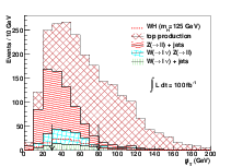
(a) pmissT after all other cuts. |
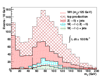
(b) mT after all other cuts. |
| Selection | NsWH | N bWH | N
sWH∕ |
| pT lW > 25 GeV, p T τl,τh > 15 GeV, ∑q l = ±1 and no jet | 233 | 171408 | 0.6 |
| 30 < Emiss T < 80 GeV | 137 | 19124 | 1.0 |
| mT > 50 GeV | 103 | 1582 | 2.6 |
| No opposite-sign same-flavour lW τl | 92 | 1177 | 2.7 |
| Process | Number of events |
| t(→ lνlνb) | 573 |
| Z∕γ∗(→ ll) + 1 jet | 330 |
| tW(→ lνblν) | 112 |
| W(→ lν)Z∕γ∗(→ ττ) | 81 |
| W(→ lν) + 2 jets | 52 |
| W(→ lν)Z∕γ∗(→ ee∕μμ) | 30 |
| Total | 1177 |
Production of a Higgs boson in association with a Z boson has a lower production cross section than WH but has the advantage that it is less susceptible to backgrounds with fake τh production. The final state particle combinations considered are summarised in Table 5.9, where two of the light leptons must be of the same flavour and opposite charge. Note that events where both taus decay hadronically are considered.
| Case | Process | Final state |
| i | Z(→ l±l∓)τ±(→ τ h±ν)τ∓(→ τ h∓ν) | two leptons, two τ h and pmiss T |
| ii | Z(→ l±l∓)τ±(→ l±2ν)τ∓(→ τ h∓ν) | three leptons, one τ h and pmiss T |
The ZH channels have relatively low signal statistics in 100 fb−1 of integrated luminosity, with an irreducible dominant background from ZZ production. Therefore, loose selection requirements are applied and the channels are combined. Additional sensitivity could be achieved by incorporating the lZlZτlτl channel, but it is not considered here because of the small branching ratio and the increased ZZ background.
While the dominant background is expected to come from diboson production, where two Z bosons decay leptonically (ZZ → ℓℓττ), a small yield is expected from Z +jets and t events in which two jets have been mis-identified as hadronically decaying tau leptons in Case i or a light-lepton and a τh in Case ii. These backgrounds are modelled by applying the product of jet mis-identification rates listed in Table 5.3 to jet pairs in these events. Production of ZZ background and ZH signal are modelled using the trigger- and identification-corrected MC acceptances listed in Table 5.3.
The ZH signal and background process cross sections are listed in Table 5.10. Like the WH process, the ZH signal cross sections is calculated using V2HV [52] and includes QCD corrections at NLO. Background process cross sections are calculated using MCFM [54] at NLO applying the same generator cuts as the WH backgrounds.
| mH (GeV) | σ(pp → ZH) | BR(H → ττ) |
| 115 | 1.05 pb | 0.0739 |
| 120 | 0.922 pb | 0.0689 |
| 125 | 0.813 pb | 0.0620 |
| 130 | 0.718 pb | 0.0537 |
| 135 | 0.638 pb | 0.0444 |
| Background process | σ × BR
| |
| Z∕γ∗(→ ℓℓ)Z∕γ∗(→ ττ) | 17.7 pb × 0.340% = 60.2 fb
| |
| Z(→ ℓℓ∕ττ) + 2 jets | 9018 pb × 10.1% = 911 pb
| |
| t → ℓνℓνb | 933 pb × 10.4% = 97.9 pb
| |
Due to the neutrinos produced in each tau decay, a conventional mass reconstruction is not possible. However, since the physical sources of missing momentum originate from the Higgs boson decay, the collinear mass approximation (see Chapter 7) can be used to reconstruct the Higgs boson mass.
The highest (lowest) pT lepton from the decay is required to have pT > 25 (15) GeV. Events
are selected by first requiring an opposite-charge same-flavour lepton pair; these are the Z decay
products. In events with three light-leptons, the opposite-sign same-flavour lepton pair with an
invariant mass closest to the Z boson mass are assumed to originate from the Z boson decay.
The remaining object pair (τlτh or τlτl) is assumed to originate from the Higgs decay
and are also required to be of opposite charge. Table 5.11 shows the numbers of signal
(NsZH) and background (N
bZH) events, as well as N
sZH∕ , in each channel, after
each selection requirement. The collinear mass requirement reduces the signal yield by
nearly 20%; recovering these events with an alternative mass variable would improve the
measurement.
, in each channel, after
each selection requirement. The collinear mass requirement reduces the signal yield by
nearly 20%; recovering these events with an alternative mass variable would improve the
measurement.
Using these selection criteria, the expected number of signal and background events for the final states listed in Table 5.9 are shown in Tables 5.12 and 5.13. The signal and background collinear mass distributions of events passing the full event selections are shown in Figure 5.3.2 for Case i and Case ii events.
| Selection | NsZH | N bZH | N
sZH∕ |
| Opposite-charge τhτh and lZlZ; | |||
| highest (lowest) pT lZ > 25 (15) GeV; p T τh > 25 GeV | 32 | 193 | 2.3 |
| Collinear mass solution | 26 | 144 | 2.1 |
| Opposite-charge τhτl and lZlZ; | |||
| highest (lowest) pT lZ > 25 (15) GeV; p T τh(τl) > 25 (15) GeV | 36 | 266 | 2.2 |
| Collinear mass solution | 30 | 188 | 2.2 |
The last set of associated Higgs production channels considered are those with a t pair. In particular, when the t pair decays semi-leptonically, t → ℓνq′b, the final states are the same as that of a WH analysis with the addition of 2 light jets and 2 b-jets. The final states considered are summarised in Table 5.14. Due to the high multiplicity of the final state and the presence of at least one lepton resulting from the decay of a top quark, the H → ττ → τhτh2ν decay is not overwhelmed by SM backgrounds and is also considered.
| Case | Process | Final state |
| iii | t(→ qbl±ν)τ±(→ τ h±ν)τ∓(→ τ h∓ν) | one lepton, two τ h, 4 jets and pmiss T |
| iv | t(→ qbl±ν)τ±(→ l±2ν)τ∓(→ τ h∓ν) | two leptons, one τ h, 4 jets and pmiss T |
The dominant background is expected to come from t(→ lνq′b)Z∕γ∗ where the Z∕γ∗ decays to a pair of leptons. A small contribution is also expected from t +jets and W(→ ℓν) +6 jets where two jets are mis-identified as a pair of τh in Case iii or a light-lepton and a τh in Case iv. These backgrounds are modelled by allowing jet pairs to be mis-identified as a pair of τh or a lepton and a τh, and weighting the event by the product of each jet mis-identification rate shown in Table 5.3. The tZ∕γ∗ background and tH signal are modelled using the trigger- and identification-corrected MC acceptances listed in Table 5.3.
The tH signal and background cross sections are summarised in Table 5.15. The tH signal cross section is calculated with NLO QCD corrections [55]. Alpgen is used to calculate the cross section of W + 6 jets and t + 2 jets.
| mH (GeV) | σ(pp → tH) | BR(H → ττ) |
| 115 | 0.785 pb | 0.0739 |
| 120 | 0.694 pb | 0.0689 |
| 125 | 0.623 pb | 0.0620 |
| 130 | 0.559 pb | 0.0537 |
| 135 | 0.501 pb | 0.0444 |
| t(→ lνqb)Z∕γ∗(→ ee∕μμ) | 973 fb × 2.89% = 28.1 fb
| |
| t(→ lνqb)Z∕γ∗(→ ττ) | 973 fb × 1.45% = 14.1 fb
| |
| t(→ lνqb) + 2 jets | 255 pb × 43.8% = 112 pb
| |
| W(→ ℓν) + 6 jets | 23.5 pb × 32.4% = 7.61 pb
| |
As with the WH selection, ℓW from the semi-leptonic top quark decay is defined to be the highest pT lepton (pT ℓW > p T τℓ) and in Case iv events, τ l is therefore defined as the lower pT lepton. The leptonic W decay and each τ decay will produce neutrinos. Therefore, the visible mass of the τlτh (τhτh) pair is used in a binned-likelihood fit to extract the signal yield of each channel.
To suppress the tZ background, events with an opposite-charge same-flavour lepton pair in Case iv events are removed if they have |mZ − mℓℓ| < 10 GeV (Figure 5.3.3). The two τh candidates and the τh −τℓ in Cases iii and iv, respectively, are required to be oppositely charged to reduce the background from mis-identified jets. To suppress the contribution from t +jets, the visible mass is required to be less than 150 GeV.
Using these selection criteria, the expected number of signal and background events for the final states listed in Table 5.14 are shown in Tables 5.16 and 5.17. The signal and background visible mass distributions of events passing the full event selection in Case iii and Case iv events are shown in and Figures 5.5(a) and 5.5(b), respectively.
| mH (GeV) | Channel | NsttH | N
sttH∕ |
| 115 | t + τ hτl | 47 | 4.8 |
| t + τ hτh | 17 | 2.7 | |
| 120 | t + τ hτl | 47 | 4.8 |
| t + τ hτh | 16 | 2.5 | |
| 125 | t + τ hτl | 37 | 3.7 |
| t + τhτh | 14 | 2.1 | |
| 130 | t + τhτl | 30 | 3.0 |
| t + τhτh | 11 | 1.7 | |
| 135 | t + τhτl | 22 | 2.2 |
| t + τhτh | 7 | 1.1 | |
| Process | t + τhτl | t + τhτh |
| channel | channel | |
| t(→ lνlνb) + 3 jets | 52 | 20 |
| t(→ lνqb) + Z∕γ∗(→ ee∕μμ) | 32 | 2 |
| t(→ lνqb) + Z∕γ∗(→ ττ) | 13 | 5 |
| t(→ lνqb) + 2 jets | 2 | 15 |
| Total | 99 | 42 |
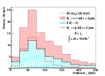
(a) tH τhτh visible mass distribution. |
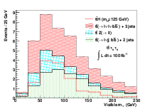
(b) tH τℓτh visible mass distribution. |
After applying the full event selection, the sensitivity of each channel is evaluated by extracting the number of expected signal events from a binned-likelihood fit. The expected variation of measurements is determined using an ensemble of pseudo-experiments of the mass-based distribution of each channel.
Expected sensitivities oo the cross section of a given process is determined using
pseudoexperiments . In each pseudoexperiment, data are produced according to a Poisson
distribution in each bin of the relevant mass-based fit distribution, where the mean of the Poisson
is equal to the expected number of signal and background events in that bin. The number of signal
events is determined by minimizing the negative log likelihood of the fit distribution. This
procedure is performed for 104 pseudoexperiments for each process, and the statistical uncertainty
is taken to be the root-mean square of the resulting signal-yield distribution. The relative
statistical uncertainty on the σ × BR of each signal process are shown in Figure 5.6. Sub-channels
are combined according to 1∕σ = 1∕ . Since the ratio of the WWH and ZZH
couplings are fixed by the SU(2)L gauge symmetry of the SM, the WH and ZH channels are
combined into the V H channel.
. Since the ratio of the WWH and ZZH
couplings are fixed by the SU(2)L gauge symmetry of the SM, the WH and ZH channels are
combined into the V H channel.
5.5 Expected sensitivity to SM Higgs coupling ratios
Measuring these channels allows us to directly probe the ΓV ∕Γt ratio. The expected uncertainty on this ratio for a range of SM Higgs boson masses and detector conditions is shown in Figure 5.7, assuming the expected sensitivity of each of the WH, ZH and tH sub-channels shown in Figure 5.6.
Recent predictions of the expected LHC sensitivity to the processes σ(pp → V H(→ b)) [20]
and σ(pp → tH(→ b)) [55, 56, 57] determine a signal sensitivity NS∕ for a range of
SM Higgs boson masses. By taking the inverse of this signal significance as the expected
relative uncertainty of a measurement of the σ × BR of these channels (assuming no
systematic uncertainties) an estimate of the expected uncertainty on a measurement
of Γτ∕Γb using both production mechanisms is made. This is shown as a function of
SM Higgs boson mass, assuming the sensitivity of each sub-channel shown in Figure
5.7.
for a range of
SM Higgs boson masses. By taking the inverse of this signal significance as the expected
relative uncertainty of a measurement of the σ × BR of these channels (assuming no
systematic uncertainties) an estimate of the expected uncertainty on a measurement
of Γτ∕Γb using both production mechanisms is made. This is shown as a function of
SM Higgs boson mass, assuming the sensitivity of each sub-channel shown in Figure
5.7.
The associated SM Higgs production channels WH, ZH and tH can be used to probe the Yukawa coupling strength gττH and the coupling ratios Γτ∕Γb and ΓV ∕Γt. With an integrated luminosity of 100 fb−1, experiments at the LHC are expected to be sensitive to these coupling ratios, with an expected relative uncertainty of 20% - 50%, depending on the SM Higgs boson mass and the detector performance.
Chapter 6
Tau identification and mis-identification probability 6.1 Introduction
This chapter describes the physics of hadronic tau decay (τh) and τh reconstruction and identification in ATLAS. Finally, a measurement of the τh mis-identification probability for hadronic jets using data collected in 2010 is also presented.
The tau lepton was first discovered in experiments at the SPEAR e+e− collider experiment at SLAC in 1974 as an excess of events with an opposite sign electron-muon pair with large missing energy [6]. The tau rest mass has since been measured to a high degree of accuracy to be 1776±0.17 MeV1 1In natural units where c = 1. with a mean lifetime, τ = (290.6 ± 1.0) × 10−15 s leading to an average decay length cτ = 87.11 μm [6]. Tau leptons decay weakly and the experimental signature can be classified as either ‘leptonic’, where either an electron or muon is produced through the decay of a virtual W boson, or ‘hadronic’ where one or more charged and neutral mesons can be detected, as shown in Figure 6.1(a). Both of these classes of tau decay cause an observed momentum imbalance due to the undetected neutrino(s) produced in the tau decay.
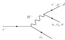
(a) Possible Tau decay diagrams. |
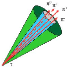
(b) A hadronically decaying tau lepton
illustration. |
No distinction is made in ATLAS between a measured ‘primary’ lepton such as those produced in Z → e+e−∕μ+μ− decay or a measured lepton produced in tau decay. The branching fractions of the leptonic and hadronic final states of tau decay have also been measured previously; the corresponding final states identified in ATLAS are shown in Table 6.1. The hadronic final states are classified into cases where either one or three reconstructed charged particle tracks are produced, since the tau lepton is electromagnetically charged with |Q| = 1. This covers about 98% of all possible hadronic tau decays.
| τ− Final State | BR (%) | Decay type |
| e−ντ | 17.85 |
leptonic |
| μ−ντ | 17.36 | |
| π−ντ | 10.91 |
hadronic, 1-track |
| π−π0ντ | 25.51 | |
| π−2π0ντ | 9.29 | |
| π−3π0ντ | 1.04 | |
| K−ντ + Neutrals | 1.57 | |
| π+2π−ντ | 9.32 |
hadronic, 3-track |
| π+2π−ντπ0 | 4.61 | |
| π+K−π−ντ + Neutrals | 0.48 | |
6.3 Hadronic tau reconstruction and identification in ATLAS
Due to the Lorentz boost produced by the large mass difference between the tau lepton and its parent (typically a W or Z boson), hadronically decaying tau leptons are observed as narrow, pencil-like hadronic jets with one or three tracks, as shown in Figure 6.1(b).
A description of τh reconstruction is given in Section 3.7.6.
Every reconstructed hadronic jet will seed a corresponding τh candidate, offering no background rejection. The following variables are used to provide separation between true τh and hadronic jets where all energies are calibrated at the EM scale:
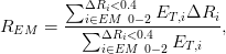 | (6.1) |
where i is the index over EM calorimeter cells associated with the τh candidate (and hence its seed jet) in the pre-sampler and layers 1 and 2. The angular separation between the calorimeter cell and the τh axis is ΔRi, and ET,iEM is the cell transverse energy.
 | (6.2) |
where the index i is over the hadronic calorimeter cells and the cells in layer 3 of the EM calorimeter that are associated with the seed jet.
R
track =  ,(6.3)
where the index i runs over all inner detector tracks passing the selection criteria in
Section 3.7.6 within a cone of ΔR = 0.4 from the τh axis and pTi is the p
T of track
i.
Leading track momentum fraction (ftrack): ,(6.3)
where the index i runs over all inner detector tracks passing the selection criteria in
Section 3.7.6 within a cone of ΔR = 0.4 from the τh axis and pTi is the p
T of track
i.
Leading track momentum fraction (ftrack):
where pT
where i and j are the indices over all calorimeter cells associated with the τh candidate (and
hence its seed jet) within a cone of radius ΔR = 0.1 and ΔR = 0.4 from the jet-axis,
respectively.
Calorimeter radius (R
| |||||||||||||||||||||||||||||||||||||||||||||||||||||||||||||||||||||||||||||||||||||||||||||||||||||||||||||||||||||||||||||||||||||||||||||||||||||||||||||||||||||||||||||||||||||||||||||||||||||||||||||||||||||||||||||||||||||||||||||||||||||||||||||||||||||||||||||||||||||||||||||||||||||||||||||||||||||||||||||||||||||||||||||||||||||||||||||||||||||||||||||||||||||||||||||||||||||||||||||||||||||||||||||||||||||||||||||||||||||||||||||||||||||||||||||||||||||||||||||||||||||||||||||||||||||||||||||||||||||||||||||||||||||||||||||||||||||||||||||||||||||||||||||||||||||||||||||||||||||||||||||||||||||||||||||||||||||||||||||||||||||||||||||||||||||||||||||||||||||||||||||||||||||||||||||||||||||||||||||||||||||||||||||||||||||||||||||||||||||||||||||||||||||||||||||||||||||||||||||||||||||||||||||||||||||||||||||||||||||||||||||||||||||||||||||||||||||||||||||||||||||||||||||||||||||||||||||||||||||||||||||||||||||||||||||||||||||||||||||||||||||||||||||||||||||||||||||||||||||||
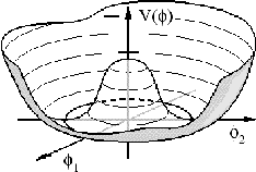
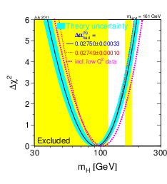
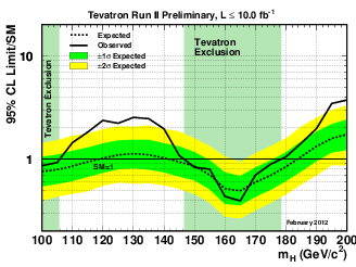
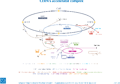
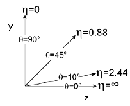
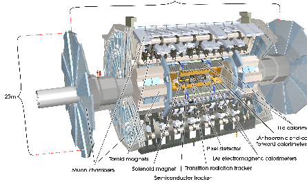
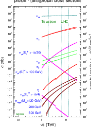
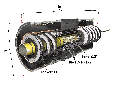
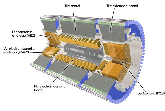
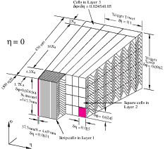
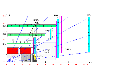
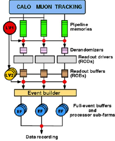
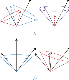
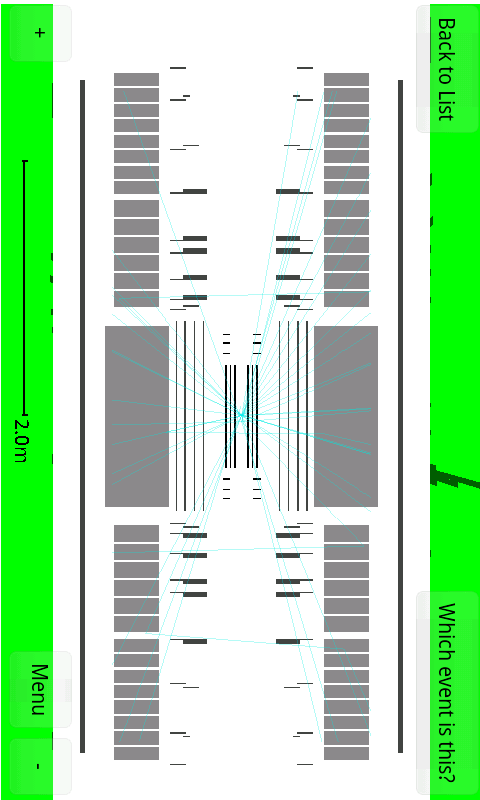
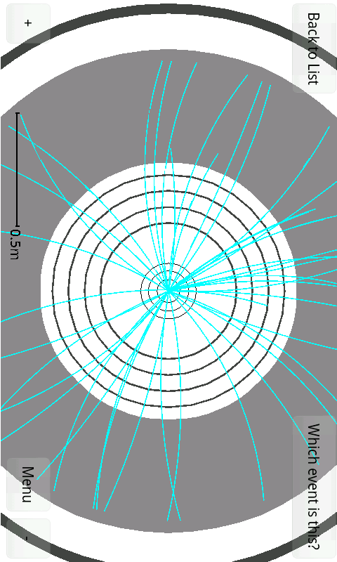
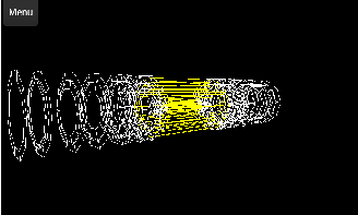
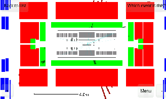
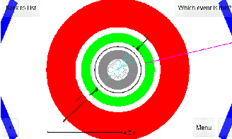
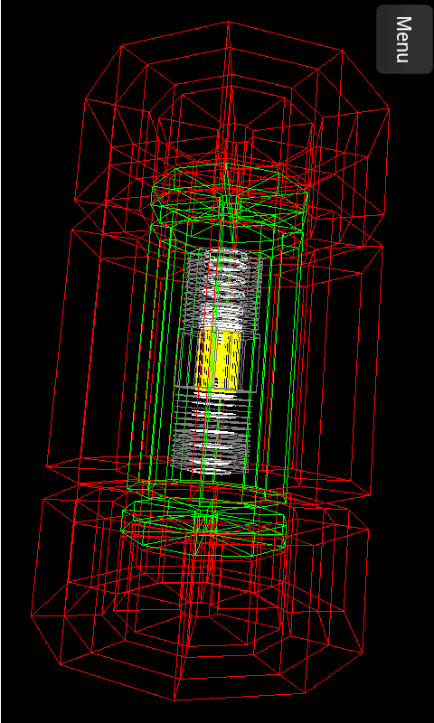
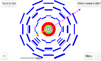
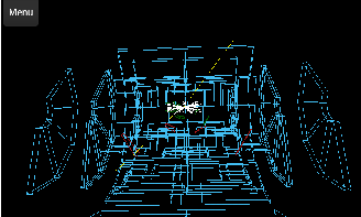
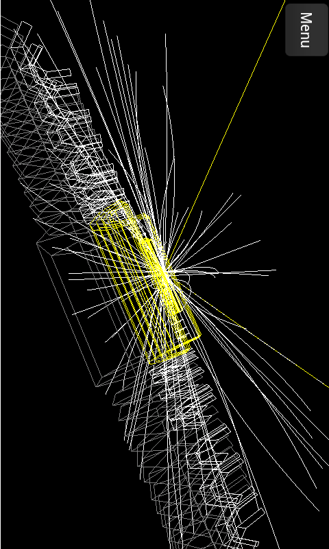
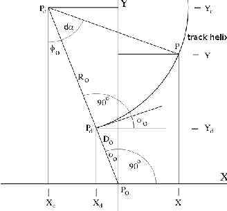

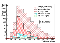

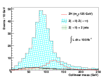
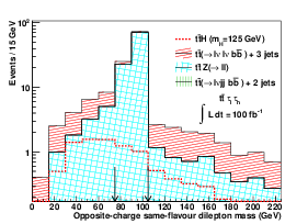
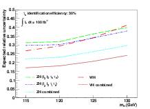
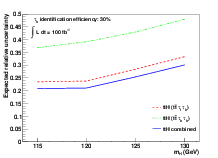
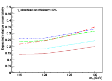
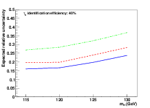
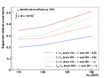
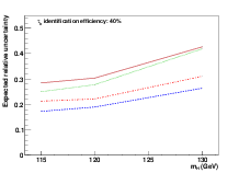
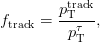
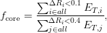

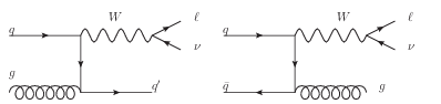

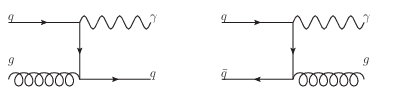
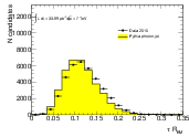
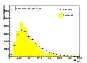
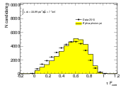
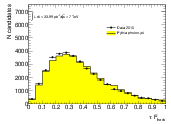
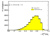
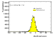
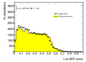
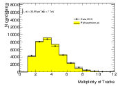
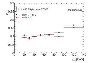
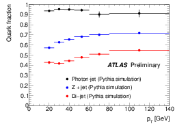
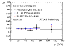

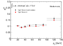
 ). The
deviation of Δ
). The
deviation of Δ ,
,  .
. 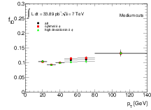
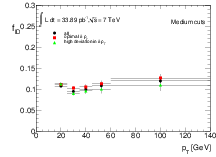
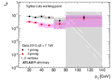
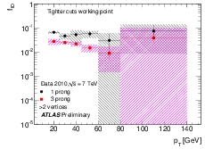
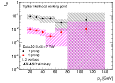
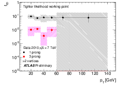
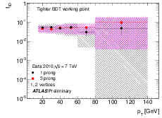

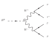
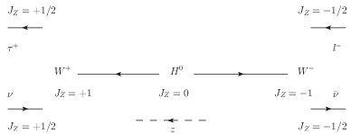
 = 7
= 7
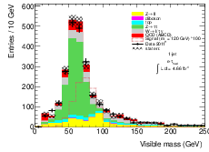
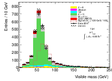


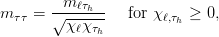
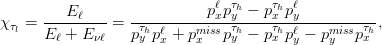
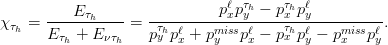
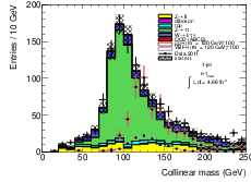
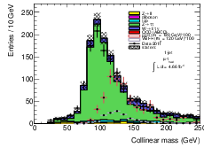


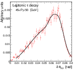
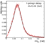
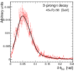
 ˙miss1,2


 = 0
= 0 where
where 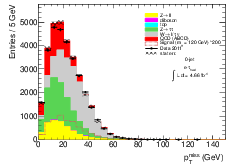
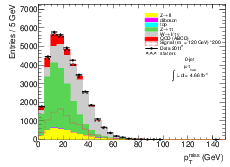
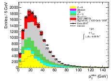
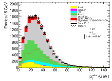
![∘ ----------------------------
ℓ miss miss
mT = 2pTpT (1 − cos Δϕ [ℓ,pT ]),](thesis199x.png)
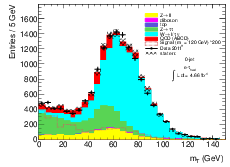
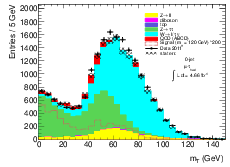
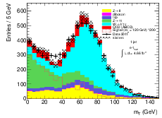
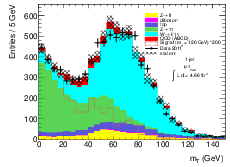
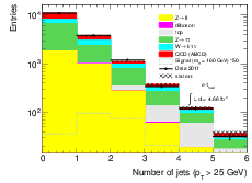
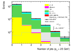

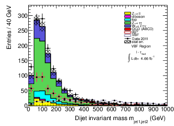
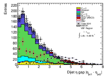
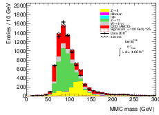
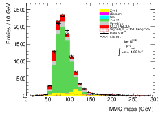
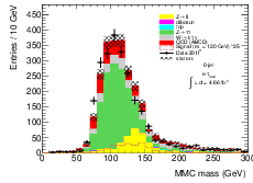
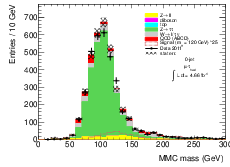
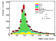
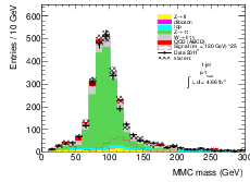
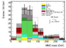

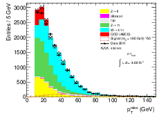
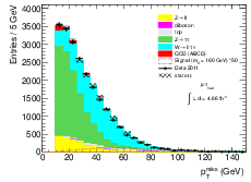
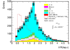
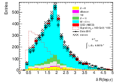
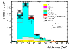
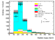

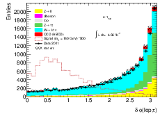
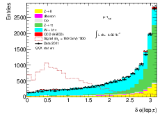

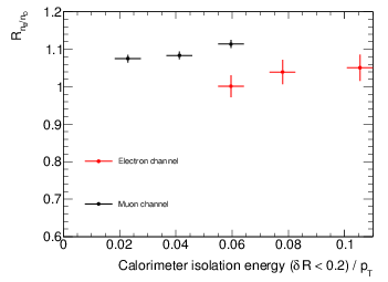

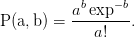


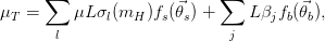

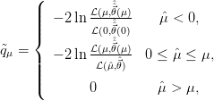
 is the maximum likelihood estimator of
  represents the nuisance parameters evaluated at
  (
( at a given
 (
(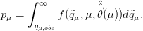
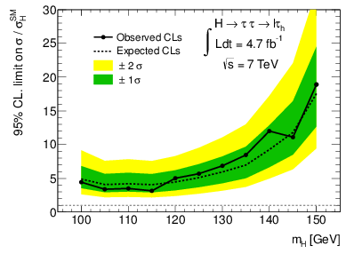
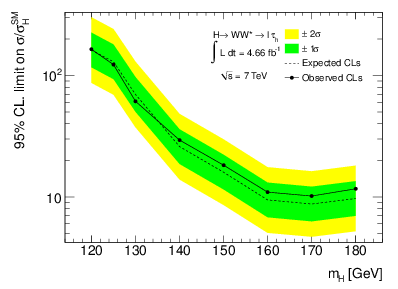
 = 8
= 8 = 7
= 7 = 7
= 7

 = 7 TeV
using the ATLAS Detector in 2011. Technical Report ATLAS-COM-CONF-2011-130,
CERN, Geneva, Jul 2011.
[73]
= 7 TeV
using the ATLAS Detector in 2011. Technical Report ATLAS-COM-CONF-2011-130,
CERN, Geneva, Jul 2011.
[73]